Table of contents *

1 Abstract *

2 Introduction *

3 Analysis of the simple fin 2D and 3D *

4 Analytical solution *

5 Fin with core *

6 Analysis of fin with core 1; K = 25 *

7 Analysis of core 2; K = 100 *

8 Discussion *

The simple fin *

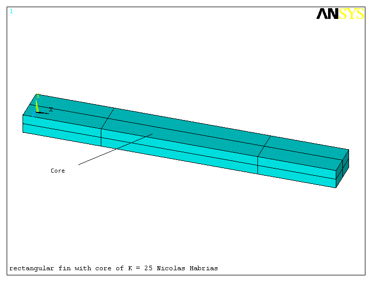
The mesh *

Temperature distribution – core 1 K=25 *

Temperature distribution – core 2 K=100 *

9 Conclusion *

Appendix – Log file for fin with core 1 ( K/2 ) *

This report deals with an ANSYS investigation into the thermal analysis of a rectangular fin. We considered three fins of the same dimension. The first fin had some uniform material properties. The two other fins had a core inside with different properties. An appropriate mesh was designed for each of these cases, and an analysis was carried out. The ANASYS solution was compared to the analytical solution. This showed the accuracy of the ANSYS solution.

I apologise not printing my report in colour but I used the printer in room M107 that is not a colour printer for economical reasons. Nevertheless I think that the quality of the graphs is quite good all the same.

The thermal stress is a very important consideration when examining the possibility of failure in component. Material strength can be greatly affected by high temperature, but even at lower temperature a high temperature gradient can produce stress. Therefore it is important to be able to analysis thermal stresses in a body.

The aim of this investigation was to examine the temperature, his gradient and the thermal stress in a rectangular fin. This fin had dimensions of 800 * 200 * 100 ( mm * mm * mm ).

The important factors considered were the temperature distribution along the central axis of the fin and the heat transfer from the fin. The conditions given were:

• Root temperature = 180 ° C
• Ambient temperature = 25 ° C

Three bars were examined. The first was a solid bar of uniform material properties, given as:

• Thermal conductivity = 50 W/mK
• Surface heat transfer coefficient = 90 W/m^2K

The second and third fins both contained a core that had material properties different from the rest of the bar. The two cores were geometrically identical, but had different thermal conductivity. The dimensions of the core were 400 * 100 * 50 (mm * mm * mm ). The core was centrally located. The thermal conductivity of the two cores were given as:

• Core1 – Thermal conductivity = 25 W/mK
• Core2 – Thermal conductivity = 100 W/mK

The simple fin was examined first. As the fin is symmetrical, only one quarter of the fin was modelled. The symmetrical planes were considered adiabatic, which simplified the analysis.

The 2D geometry was set up and mesh, using the LESIZE command. Several meshes were tried, but the difference in results proved to be negligible. The VDRAG command was used to create the 3D model. The base temperature was applied to the end of the fin, and the convection conditions were applied to the outer surfaces. Then the model was solved.

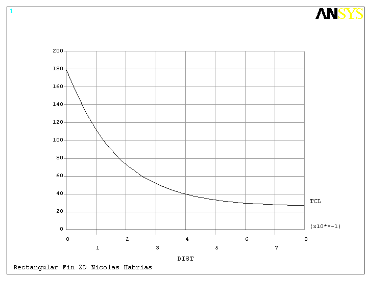
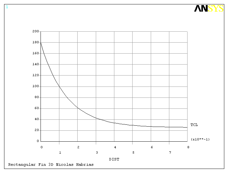
Firstly the temperature distributions was displayed as graph 1 ( 2D ) and graph 2 ( 3D ).

These graph show that the temperature at the end of the fin is much higher than the ambient temperature. Two methods of analytical solution exist. One considers the fin infinitely long. A fin can be considered infinitely long when the temperature at the end of the bar is the same as the ambient temperature. The ANSYS results show that this is not true. Consequently, the fin must be considered as a short fin.

When we compare both graphs, we find different temperatures at the end of the fins ( 27.041° C for the 2D fin and 25.717° C for the 3D fin ). Furthermore the forms of the graphs are different.

Consequently, the hypotheses of a 2D fin is incorrect and we must study the 3D fin.

The validity of the ANSYS results was then analysed by comparing them to the analytical solution.

The calculation shown below verifies the previous assumption that the fin can be considered "short". So, heat loss in a short bar is given by:

Heat loss in an infinitely long fin is given by:

Where:

h= 90 W/mK k= 50 W/m²K q _b= 180 C A=0.02 m² P=0.6 m

L= 0.8

By equating these two expressions the minimum length of fin that can be considered infinitely long can be calculated.

So:

For the conditions and properties given, a minimum length of 360 mm is required. However, we can not say that the bar is infinitely long because the temperature at the end of the bar is not equal to then ambient temperature. Furthermore 800 is not far from 360 mm. For example, a long bar would have a length of at least 10 m. Finally we keep the hypotheses of a long bar.

With:

• q = difference of temperature with the ambient at x
• q _b = difference between source temperature and ambient temperature
• x = distance along fin

The temperature distribution was calculated using the analytical solution, in order to see the differences. The analytical solution can be found in the table below.

It can be seen that the ANSYS and analytical solution compare closely. The temperature at the end of the bar given by ANSYS was 25.717. These results give a difference of 0.87 – 0.717 » 0.15 ° C. So for the temperature distribution, the results are good.

Heat loss:

Finally, this gives a calculated heat loss of 1.322 kW.

As with the simple fin, only one quarter of the fin was modelled for reasons of symmetry.

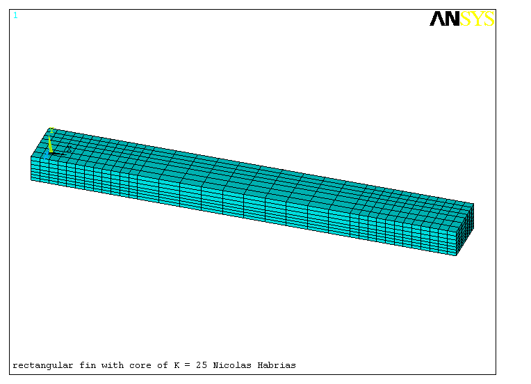The volumes were then created using the VDRAG command. The 2D were first dragged along a line equivalent to the width of the core. This was done to create the core ( graph 3 and graph 4 ). The areas were then dragged a second time to create the total volume. The NUMMRG command was utilised after the volumes had been created to ensure that all the nodes had completely merged together. The two different material properties were there defined and applied to the relevant volumes. Finally the convection properties and root temperature were applied. The model was then ready to be solved. The complete log file can be found in appendix.

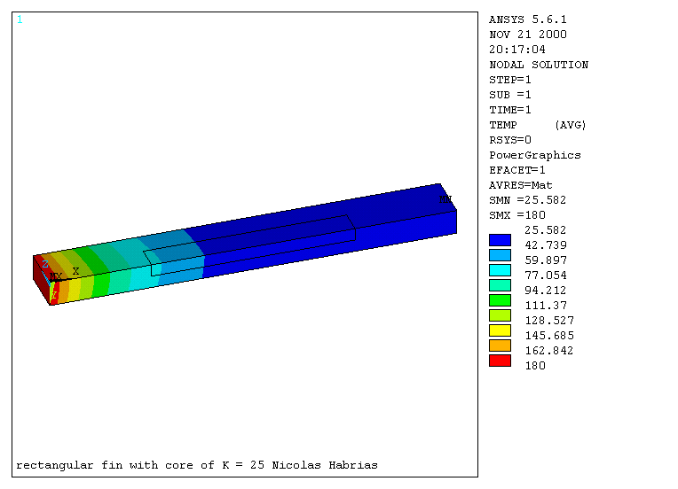The effects on the two different cores were examined separately. Core 1 has a thermal productivity of 25 W/mK, i.e. half of the rest of the fin. Firstly the temperature distribution along the length of the film was examined. The contour plot of the nodal solution can be found in graph 5. If we do a zoom we can see that the temperature distribution is a very little affected around the core area.

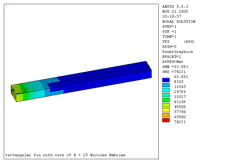For a more detailed examination, the thermal flux in the x-direction was examined. This plot can be found in graph 6. This plot shows clearly the effect of the different thermal conductivity of the core.

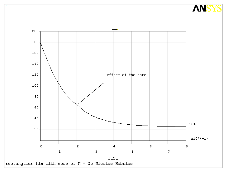The overall temperature distribution was then plotted in graph 7 to show exactly how the core affects the temperature along the length.

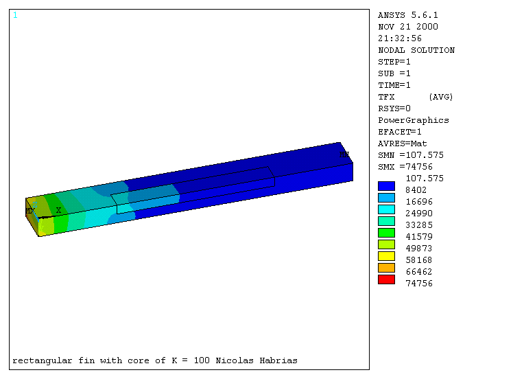
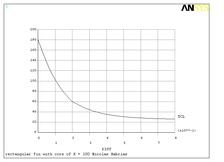
The core 2 had a thermal conductivity of 100 W/mK which is twice that of the rest of the fin. The contour plot of the nodal solution can be found in graph 8. The thermal flux in the x-direction can be found in graph 9. The overall temperature distribution was then plotted in graph 10.

Graph 10

The results obtained for the simple fin are nearly similar to the analytical results. The error between the 2 methods for the temperature at the end of the fin is 0.6%. So there is a close correlation between the two methods.

We made an accurate mesh at the beginning of the fin because the heat is applied at this area. Like that the calculation is more accurate were the heat is maximum.

The core 1 has a thermal conductivity of half of the rest of the fin. Consequently, the thermal flux is lower in the core so the temperature decreases slower in the core. This produces the effect displayed in the curve at this point.

The temperature does not change with the core and without the core because we consider a static problem and because there are some exchanges between the core and the rest of the fin.

The core 2 has a thermal conductivity twice of the rest of the fin. Consequently, the thermal flux is higher in the core. The temperature decreases faster in the core. This produces a dip in the temperature distribution curve.

Last but not least, the more the thermal conductivity is high, the more the heat is allowed to move and the more the temperature decreases.

In conclusion, this ANSYS investigation gave good results in comparison with the analytical solutions. Finally, ANSYS is a very useful software to solve thermal problems. Nevertheless, it’s a shame that ANSYS could not mesh directly in 3D with bricks when we consider a thermal problem. Indeed the meshing in 2D using LESIZE is quite long.